

文章转自ADI官网,版权归属原作者一切
In applications that use filters, the amplitude response is generally of greater interest than the phase response. But in some applications, the phase response of the filter is important. An example of this might be where a filter is an element of a process control loop. Here the total phase shift is of concern, since it may affect loop stability. Whether the topology used to build the filter produces a sign inversion at some frequencies can be important.
It might be useful to visualize the active filter as two cascaded filters. One is the ideal filter, embodying the transfer equation; the other is the amplifier used to build the filter. This is illustrated in Figure 1. An amplifier used in a closed negative-feedback loop can be considered as a simple low-pass filter with a first-order response. The gain rolls off with frequency above a certain breakpoint. In addition, there will be, in effect, an additional 180° phase shift at all frequencies if the amplifier is used in the inverting configuration.

First, the filter response is chosen; then, a circuit topology is selected to implement it. The filter response refers to the shape of the attenuation curve. Often, this is one of the classical responses such as Butterworth, Bessel, or some form of Chebyshev. Although these response curves are usually chosen to affect the amplitude response, they will also affect the shape of the phase response. For the purpose of the comparisons in this discussion, the amplitude response will be ignored and considered essentially constant.
Filter complexity is typically defined by the filter “order,” which is related to the number of energy storage elements (inductors and capacitors). The order of the filter transfer function’s denominator defines the attenuation rate as frequency increases. The asymptotic filter rolloff rate is –6n dB/octave or –20n dB/decade, where n is the number of poles. An octave is a doubling or halving of the frequency; a decade is a tenfold increase or decrease of frequency. So a first-order (or single-pole) filter has a rolloff rate of –6 dB/octave or –20 dB/decade. Similarly, a second-order (or 2-pole) filter has a rolloff rate of –12 dB/octave or –40 dB/decade. Higher-order filters are usually built up of cascaded first- and second-order blocks. It is, of course, possible to build third- and, even, fourth-order sections with a single active stage, but sensitivities to component values and the effects of interactions among the components on the frequency response increase dramatically, making these choices less attractive.
The Transfer Equation
First, we will take a look at the phase response of the transfer equations. The phase shift of the transfer function will be the same for all filter options of the same order. For the single-pole, low-pass case, the transfer function has a phase shift, Φ, given by
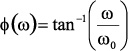 |
(1) |
where:
ω = frequency (radians per second)
ω0 = center frequency (radians per second)
Frequency in radians per second is equal to 2π times frequency in Hz (f), since there are 2π radians in a 360° cycle. Because the expression is a dimensionless ratio, either f or ω could be used.
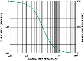
The center frequency can also be referred to as the cutoff frequency (the frequency at which the amplitude response of the single-pole, low-pass filter is down by 3 dB—about 30%). In terms of phase, the center frequency will be at the point at which the phase shift is 50% of its ultimate value of –90° (in this case). Figure 2, a semi-log plot, evaluates Equation 1 from two decades below to two decades above the center frequency. The center frequency (=1) has a phase shift of –45°.
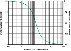
Similarly, the phase response of a single-pole, high-pass filter is given by:
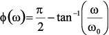 |
(2) |
Figure 3 evaluates Equation 2 from two decades below to two decades above the center frequency. The normalized center frequency (=1) has a phase shift of +45°.
It is evident that the high-pass and the low-pass phase responses are similar, only shifted by 90° (π/2 radians).

For the second-order, low-pass case, the transfer function has a phase shift that can be approximated by
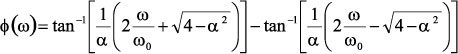 |
(3) |
where α is the damping ratio of the filter. It will determine the peaking in the amplitude response and the sharpness of the phase transition. It is the inverse of the Q of the circuit, which also determines the steepness of the amplitude rolloff or phase shift. The Butterworth has an α of 1.414 (Q of 0.707), producing a maximally flat response. Lower values of α will cause peaking in the amplitude response.
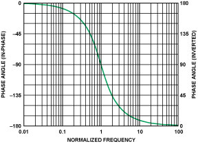
Figure 4 evaluates this equation (using α = 1.414) from two decades below to two decades above the center frequency. Here the center frequency (=1) shows a phase shift of –90°.The phase response of a 2-pole, high-pass filter can be approximated by
 |
(4) |
In Figure 5 this equation is evaluated (again using α = 1.414), from two decades below to two decades above the center frequency (=1), which shows a phase shift of –90°.
Again, it is evident that the high-pass and low-pass phase responses are similar, just shifted by 180° (π radians).
In higher-order filters, the phase response of each additional section is cumulative, adding to the total. This will be discussed in greater detail later. In keeping with common practice, the displayed phase shift is limited to the range of ±180°. For example, –181° is really the same as +179°, 360° is the same as 0°, and so on.
First-Order Filter Sections
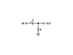
First-order sections can be built in a variety of ways. The most straightforward way is illustrated in Figure 6, simply using a passive R-C configuration. The center frequency of this filter is 1/(2πRC). It is commonly followed by a noninverting buffer amplifier to prevent loading by the circuit following the filter, which could alter the filter response. In addition, the buffer can provide some drive capability. The phase will vary with frequency as shown in Figure 2, with 45° phase shift at the center frequency, exactly as predicted by the transfer equation, since there are no extra components to modify the phase shift. That response will be referred to as the in-phase, first-order, low-pass response. The buffer will add no phase shift, as long as its bandwidth is significantly greater than that of the filter.
Remember that the frequency in these plots is normalized, i.e., the ratio to the center frequency. If, for example, the center frequency were 5 kHz, the plot would provide the phase response to frequencies from 50 Hz to 500 kHz.
An alternative structure is shown in Figure 7. This circuit, which adds resistance in parallel to continuously discharge an integrating capacitor, is basically a lossy integrator. The center frequency is again 1/(2πRC). Because the amplifier is used in the inverting mode, the inversion introduces an additional 180° of phase shift. The input-to-output phase variation with frequency, including the amplifier’s phase inversion, is shown in Figure 2 (right axis). This response will be referred to as the inverted, first-order, low-pass response.
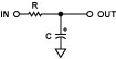
The circuits shown above, which attenuate the high frequencies and pass the low frequencies, are low-pass filters. Similar circuits also exist to pass high frequencies. The passive configuration for a first-order, high-pass filter is shown in Figure 8; and its phase variation with normalized frequency is shown in Figure 3 (in-phase response).
The plot in Figure 3 (left axis) will be referred to as the in phase, first-order, high-pass response. The active configuration of the high-pass filter is shown in Figure 9. The phase variation with frequency is shown in Figure 3 (right axis). This will be referred to as the inverted, first-order, high-pass response.

Second-Order Sections
A variety of circuit topologies exists for building second-order sections. To be discussed here are the Sallen-Key, the multiple-feedback, the state-variable, and its close cousin, the biquad. They are the most common and are relevant here. More complete information on the various topologies is given in the References.
Sallen-Key, Low-Pass Filter
The widely used Sallen-Key configuration, also known as a voltage-controlled voltage source (VCVS), was first introduced in 1955 by R. P. Sallen and E. L. Key of MIT’s Lincoln Labs (see Reference 3). Figure 10 is a schematic of a Sallen-Key, second-order, low-pass filter. One reason for this configuration’s popularity is that its performance is essentially independent of the op amp’s performance because the amplifier is used primarily as a buffer. Since the follower-connected op amp is not used for voltage gain in the basic Sallen-Key circuit, its gain-bandwidth requirements are not of great importance. This implies that, for a given op amp bandwidth, a higher-frequency filter can be designed using this fixed (unity) gain, as compared to other topologies that involve the amplifier’s dynamics in a variable feedback loop. The signal phase is maintained through the filter (noninverting configuration). A phase shift-vs.-frequency plot for a Sallen-Key, low-pass filter with Q = 0.707 (or a damping ratio, α = 1/Q of 1.414—Butterworth response) is shown in Figure 4 (left axis). To simplify comparisons, this will be the standard performance for the second-order sections to be considered here.

The Sallen-Key, High-Pass Filter
To transform the Sallen-Key low-pass into a high-pass configuration, the capacitors and the resistors in the frequency-determining network are interchanged, as shown in Figure 11, again using a unity-gain buffer. The phase shift vs. frequency is shown in Figure 5 (left axis). This is the in-phase, second-order, high-pass response.

The amplifier gain in Sallen-Key filters can be increased by connecting a resistive attenuator in the feedback path to the inverting input of the op amp. However, changing the gain will affect the equations for the frequency-determining network, and the component values will have to be recalculated. Also, the amplifier’s dynamics are more likely to need scrutiny, since they introduce gain into the loop.
The Multiple-Feedback (MFB), Low-Pass Filter
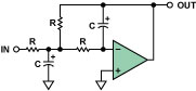
The multiple feedback filter is a single-amplifier configuration based on an op amp as an integrator (an inverting configuration) inside a feedback loop (see Figure 12). Therefore, the dependence of the transfer function on the op amp parameters is greater than in the Sallen-Key realization. It is hard to generate high-Q, high-frequency sections because of the limited open-loop gain of the op amp at high frequencies. A guideline is that the open-loop gain of the op amp should be at least 20 dB (i.e., ×10) above the amplitude response at the resonant (or cutoff) frequency, including the peaking caused by the Q of the filter. The peaking due to Q will have an amplitude of magnitude A0:
|
|
(5) |
where H is the gain of the circuit.
The multiple-feedback filter inverts the phase of the signal. This is equivalent to adding 180° to the phase shift of the filter itself. The variation of phase vs. frequency is shown in Figure 4 (right axis). This will be referred to as the inverted, second-order, low-pass response. Of interest, the difference between highest- and lowest-value components to achieve a given response is higher in the multiple-feedback case than in the Sallen-Key realization.
The Multiple-Feedback (MFB), High-Pass Filter
Comments made about the multiple-feedback, low-pass case apply to the high-pass case as well. The schematic of a multiple-feedback, high-pass filter is shown in Figure 13, and its ideal phase shift vs. frequency is shown in Figure 5 (right axis). This was referred to as the inverted, second-order, high-pass response.
This type of filter may be more difficult to implement stably at high frequencies because it is based on a differentiator, which, like all differentiator circuits, maintains greater closed-loop gain at higher frequencies and tends to amplify noise.
State-Variable
A state-variable realization is shown in Figure 14. This configuration offers the most flexible and precise implementation, at the expense of many more circuit elements, including three op amps. All three major parameters (gain, Q, and ω0) can be adjusted independently; and low-pass, high-pass, and band-pass outputs are available simultaneously. The gain of the filter is also independently variable.
Since all parameters of the state variable filter can be adjusted independently, component spread can be minimized. Also, mismatches due to temperature and component tolerances are minimized. The op amps used in the integrator sections will have the same limitations on op amp gain-bandwidth as described in the multiple-feedback section.
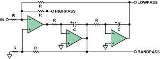
The phase shift vs. frequency of the low-pass section will be an inverted second-order response (see Figure 4, right axis) and the high-pass section will have the inverted high-pass response (see Figure 5, right axis).
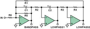
Biquadratic (Biquad)
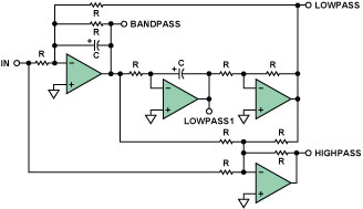
A close cousin of the state-variable filter is the biquad (see Figure 15). The name of this circuit, first used by J. Tow in 1968 (see Reference 6), and later by L. C. Thomas in 1971 (see Reference 5), is based on the fact that the transfer function is a ratio of two quadratic terms. This circuit is a slightly different form of a state-variable circuit. In this configuration, a separate high-pass output is not available. However, there are two low-pass outputs, one in-phase (LOWPASS1) and one out-of-phase (LOWPASS2).
With the addition of a fourth amplifier section, high-pass, notch (low-pass, standard, and high-pass), and all-pass filters can be realized. A schematic for a biquad with a high-pass section is shown in Figure 16.
The phase shift vs. frequency of the LOWPASS1 section will be the in-phase, second-order, low-pass response (see Figure 4, left axis). The LOWPASS2 section will have the inverted second-order response (see Figure 4, right axis). The HIGHPASS section has a phase shift that inverts (see Figure 5, right axis).
CONCLUSION
We have seen that the topology used to build a filter will have an effect on its actual phase response. This may be one of the factors used in determining the topology used. Table 1 compares the phase-shift ranges for the various low-pass filter topologies discussed in this article.
Table 1. Low-pass-filter topology phase-shift ranges.
| LOW-PASS FILTERS | ||
| FILTER TOPOLOGY | SINGLE PHASE | PHASE VARIATION |
| Single-Pole, Passive | In-Phase | 0° to –90° |
| Single-Pole, Active | Inverted | 180° to 90° |
| 2-Pole, Sallen-Key | In-Phase | 0° to –180° |
| 2-Pole, Multiple Feedback | Inverted | 180° to 0° |
| 2-Pole, State Variable | Inverted | 180° to 0° |
| 2-Pole, Biquad Lowpass1 | In-Phase | 0° to –180° |
| 2-Pole, Biquad Lowpass2 | Inverted | 180° to 0° |
Similarly, the various high-pass topologies are compared in Table 2.
Table 2. High-pass-filter topology phase-shift ranges.
| HIGH-PASS FILTERS | ||
| FILTER TOPOLOGY | SINGLE PHASE | PHASE VARIATION |
| Single-Pole, Passive | In-Phase | –90° to 0° |
| Single-Pole, Active | Inverted | –90° to –180° |
| 2-Pole, Sallen-Key | In-Phase | 180° to 0° |
| 2-Pole, Multiple Feedback | Inverted | 0° to –180° |
| 2-Pole, State Variable | Inverted | 0° to –180° |
| 2-Pole, Biquad | Inverted | 0° to –180° |
The Variation of Phase Shift with Q
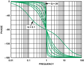
The second-order responses above have all used a Q of 0.707. Figure 17 shows the effect on phase response of a low-pass filter (the results for high-pass are similar) as Q is varied. The phase responses for values of Q = 0.1, 0.5, 0.707, 1, 2, 5, 10, and 20 are plotted. It’s worth noting that the phase can start to change well below the cutoff frequency at low values of Q.
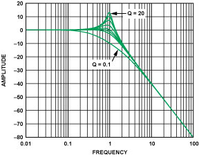
Although not the subject of this article, the variation of amplitude response with Q may also be of interest. Figure 18 shows the amplitude response of a second-order section as Q is varied over above range.
The peaking that occurs in high-Q sections may be of interest when high-Q sections are used in multistage filters. While in theory it doesn’t make any difference in which order the sections are cascaded, in practice it is typically better to place low-Q sections ahead of high-Q sections so that the peaking will not cause the dynamic range of the filter to be exceeded. Although this plot is for low-pass sections, high-pass responses will show similar peaking.
Higher-Order Filters
Transfer functions can be cascaded to form higher-order responses. When filter responses are cascaded, dB gains (and attenuations) add, and phase angles add, at any frequency. As noted earlier, multipole filters are typically built with cascaded second-order sections, plus an additional first-order section for odd-order filters. Two cascaded first-order sections do not provide the wide range of Q available with a single second-order section.
A fourth-order filter cascade of transfer functions is shown in Figure 19. Here we see that the filter is built of two second-order sections.
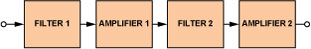
Figure 20 shows the effect on phase response of building a fourth-order filter in three different ways. The first is built with two Sallen-Key (SK) Butterworth sections. The second consists of two multiple-feedback (MFB) Butterworth sections. The third is built with one SK section and one MFB section. But just as two cascaded first-order sections don’t make a second-order section, two cascaded second-order Butterworth sections do not equal a fourth-order Butterworth section. The first section of a Butterworth filter has an f0 of 1 and a Q of 0.5412 (α = 1.8477). The second section has an f0 of 1 and a Q of 1.3065 (α = 0.7654).
As noted earlier, the SK section is noninverting, while the MFB section inverts. Figure 20 compares the phase shifts of these three fourth-order sections. The SK and the MFB filters have the same response because two inverting sections yield an in-phase response (–1 × –1 = +1). The filter built with mixed topologies (SK and MFB) yields a response shifted by 180° (+1 × –1 = –1).
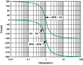
Note that the total phase shift is twice that of a second-order section (360° vs. 180°), as expected. High-pass filters would have similar phase responses, shifted by 180°.
This cascading idea can be carried out for higher-order filters, but anything over eighth-order is difficult to assemble in practice.
Future articles will examine phase relationships in band-, notch- (band-reject), and all-pass filters.
参阅电路
- Daryanani, G. Principles of Active Network Synthesis and Design. J. Wiley & Sons. 1976. ISBN: 0-471-19545-6.
- Graeme, J., G. Tobey, and L. Huelsman. Operational Amplifiers Design and Applications. McGraw-Hill. 1971. ISBN 07-064917-0.
- Sallen, R. P., and E. L. Key. “A Practical Method of Designing RC Active Filters.” IRE Trans. Circuit Theory. 1955. Vol. CT-2, pp. 74-85.
- Thomas, L. C. “The Biquad: Part II—A Multipurpose Active Filtering System.” IEEE Trans. Circuits and Systems. 1971. Vol. CAS-18. pp. 358-361.
- Thomas, L. C. “The Biquad: Part I—Some Practical Design Considerations.”IEEE Trans. Circuits and Systems. 1971. Vol. CAS-18. pp. 350-357.
- Tow, J. “Active RC Filters—A State-Space Realization.” Proc. IEEE. 1968. Vol. 56. pp. 1137-1139.
- Van Valkenburg, M. E. Analog Filter Design. Holt, Rinehart & Winston. 1982.
- Williams, A. B. Electronic Filter Design Handbook. McGraw-Hill. 1981.
- Zumbahlen, H. “Analog Filters.” Chapter 5, in Jung, W., Op Amp Applications Handbook. Newnes-Elsevier (2006).
- Zumbahlen, H. Basic Linear Design. Ch. 8. Analog Devices Inc. 2006.