


Matlab能够说是一个十分有用且功用完全的东西,在通讯、自控、金融等方面有广泛的运用。
本文评论运用Matlab对信号进行频域剖析的办法。
说到频域,不可避免的会说到傅里叶改换,傅里叶改换供给了一个将信号从时域转变到频域的办法。之所以要有信号的频域剖析,是因为许多信号在时域不明显的特征能够在频域下得到很好的展示,能够愈加简略的进行剖析和处理。
FFT
Matlab供给的傅里叶改换的函数是FFT,中文名叫做快速傅里叶改换。快速傅里叶改换的提出是巨大的,使得处理器处理数字信号的才能大大提高,也使咱们日子向数字化迈了一大步。
接下来就谈谈怎么运用这个函数。
fft运用很简略,可是一般信号都有x和y两个向量,而fft只会处理y向量,所以想让频域剖析变得有意义,那么就需求用户自己处理x向量
一个简略的比如
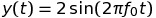
从一个简略正弦信号开端吧,正弦信号界说为:
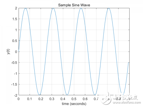
咱们现在经过以下代码在Matlab中画出这个正弦曲线
fo = 4; %frequency of the sine wave
Fs = 100; %sampling rate
Ts = 1/Fs; %sampling time interval
t = 0:Ts:1-Ts; %sampling period
n = length(t); %number of samples
y = 2*sin(2*pi*fo*t); %the sine curve
%plot the cosine curve in the TIme domain
sinePlot = figure;
plot(t,y)
xlabel(‘TIme (seconds)’)
ylabel(‘y(t)’)
TItle(‘Sample Sine Wave’)
grid
这便是咱们得到的:
当咱们对这条曲线fft时,咱们期望在频域得到以下频谱(根据傅里叶改换理论,咱们期望看见一个幅值为1的峰值在-4Hz处,另一个在+4Hz处)

运用FFT指令
咱们知道方针是什么了,那么现在运用Matlab的内建的FFT函数来从头生成频谱
%plot the frequency spectrum using the MATLAB fft command
matlabFFT = figure; %create a new figure
YfreqDomain = fft(y); %take the fft of our sin wave, y(t)
stem(abs(YfreqDomain)); %use abs command to get the magnitude
%similary, we would use angle command to get the phase plot!
%we‘ll discuss phase in another post though!
xlabel(’Sample Number‘)
ylabel(’Amplitude‘)
TItle(’Using the Matlab fft command‘)
grid
axis([0,100,0,120])
作用如下:
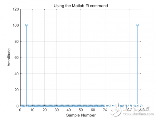
可是留意一下,这并不是咱们真实想要的,有一些信息是缺失的
x轴原本应该给咱们供给频率信息,可是你能读出频率吗?
起伏都是100
没有让频谱中心为
为FFT界说一个函数来获取双方频谱
以下代码能够简化获取双方频谱的进程,仿制并保存到你的.m文件中
function [X,freq]=centeredFFT(x,Fs)
%this is a custom function that helps in plotting the two-sided spectrum
%x is the signal that is to be transformed
%Fs is the sampling rate
N=length(x);
%this part of the code generates that frequency axis
if mod(N,2)==0
k=-N/2:N/2-1; % N even
else
k=-(N-1)/2:(N-1)/2; % N odd
end
T=N/Fs;
freq=k/T; %the frequency axis
%takes the fft of the signal, and adjusts the amplitude accordingly
X=fft(x)/N; % normalize the data
X=fftshift(X); %shifts the fft data so that it is centered
这个函数输出正确的频域规模和改换后的信号,它需求输入需求改换的信号和采样率。
接下来运用前文的正弦信号做一个简略的示例,留意你的示例.m文件要和centeredFFT.m文件在一个目录下
[YfreqDomain,frequencyRange] = centeredFFT(y,Fs);
centeredFFT = figure;
%remember to take the abs of YfreqDomain to get the magnitude!
stem(frequencyRange,abs(YfreqDomain));
xlabel(’Freq (Hz)‘)
ylabel(’Amplitude‘)
title(’Using the centeredFFT function‘)
grid
axis([-6,6,0,1.5])
作用如下:
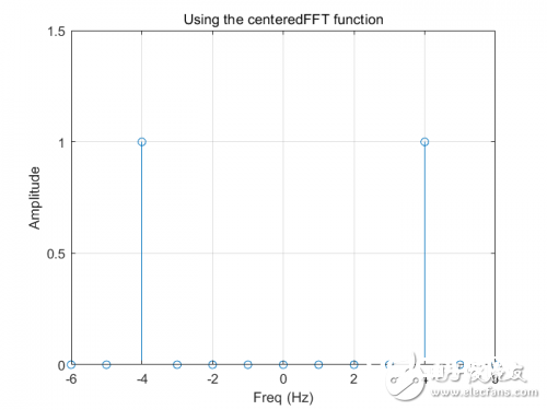
这张图就满意了咱们的需求,咱们得到了在+4和-4处的峰值,并且幅值为1.
为FFT界说一个函数来获取右边频谱
从上图能够看出,FFT改换得到的频谱是左右对称的,因而,咱们只需求其间一边就能取得信号的一切信息,咱们一般保存正频率一侧。
以下的函数对上面的自界说函数做了一些修正,让它能够协助咱们只画出信号的正频率一侧
function [X,freq]=positiveFFT(x,Fs)
N=length(x); %get the number of points
k=0:N-1; %create a vector from 0 to N-1
T=N/Fs; %get the frequency interval
freq=k/T; %create the frequency range
X=fft(x)/N; % normalize the data
%only want the first half of the FFT, since it is redundant
cutOff = ceil(N/2);
%take only the first half of the spectrum
X = X(1:cutOff);
freq = freq(1:cutOff);
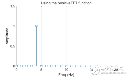
和前面相同,运用正弦信号做一个示例,下面是示例代码
[YfreqDomain,frequencyRange] = positiveFFT(y,Fs);
positiveFFT = figure;
stem(frequencyRange,abs(YfreqDomain));
set(positiveFFT,’Position‘,[500,500,500,300])
xlabel(’Freq (Hz)‘)
ylabel(’Amplitude‘)
title(’Using the positiveFFT function‘)
grid
axis([0,20,0,1.5])
作用如下: