ADI:Considering Multipliers (Part 1) [The Wit and Wisdom of Dr. Leif—7]

文章转自ADI官网，版权归属原作者一切

You may recall that Newton Leif joined Analog Devices as a young designer, bringing with him a wealth of experience and insights from his prior work. Now, in 2028, Dr. Leif continues to be active in mentoring the younger engineers at our design center located in Solna, near Stockholm. One, for whom he has a special affection, is the young Niku Chen, already well on her way to a stellar career at this company.

Throughout her life, Niku has been developing that critical aptitude—predicated on an attitude—essential for sustained success as a designer of integrated circuits: the ability to visualize, propose, promote, and then develop refreshingly novel concepts from the engineering side of the fence. In this regard, Leif’s own courageous inclination to launch ideas for long-neglected functions has been her inspiration. Time and again, the naysayers declared them to be of “no value” in the current marketplace; and yet, steadily and stealthily, he would find the resources needed to develop them.

Young Niku has this stubborn flair for imagineering from the trenches, and with but the barest of hints from Leif she’s been busy designing nanopower analog array processors for use in neuromorphic systems, employing many thousands of slow, low-accuracy, and—frankly—rudimentary multiplier cells. To the surprise of all the blind spear throwers (the most dangerous kind!), multipliers continued to be indispensable over sixty years since the very first fully monolithic ICs were fabricated in 1967 at Tektronix (for use as gain-control elements [1]) by another youthful and aspiring imagineer, to whom Dr. Leif invariably referred as “that rascally irrepressible Tinkerer.”

Cells based on the bipolar junction transistor (BJT) became the Tinkerer’s lifetime passion, after his exposure to the very first production transistors in 1954—frail, expensive little guys, and as different from one another as siblings. He joined forces with Analog Devices in 1972, and, like Niku, enjoyed the freedom to work proactively in a focused, but fiercely independent-minded and entrepreneurial, fashion. One outcome: he had proposed, and then developed, an extensive family of products loosely known as “functional” circuits—an ambiguous term, but no more so than the notion of an “operational” amplifier.

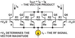
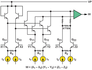
Many of these early parts were multipliers, which remained in production well into the 2010s. They exploited current-mode translinear (TL) loops [2,3,4], current-mirrors [5], and current conveyors (conceived and named by the Tinkerer during the Tektronix years), aided by linear g_m cells [6] (Figure 1). Another novel and ubiquitous cell from that era, later named a “KERMIT” [7], meaning a Kommon-EmitteR MultI–Tanh, was used as the kernel of a 2008 product, the ADL5390^† RF vector multiplier (Figure 2), and in an elaborated form in the ADL5391 dc-to-2-GHz multiplier, the latter providing exact symmetry in the time delay from its X and Y inputs, for the first time.

Today, well into the second quarter of this century, there is no disagreement, among the experts in neuromemic¹ intelligence systems, regarding the indispensable role of analog multipliers and numerous other nonlinear analog functions in this field. But at one time, during the century’s first quarter, well before the recent breakthroughs in practical neuromorphic hardware, there were legitimate reasons for doubting this outcome. Now, lacking these (the most distinctive aspect of our massively parallel hybrid, yet essentially analog, hypercessors), we’d still be squeezing miserable little on-again off-again bits through tiny pipes, a mere handful at a time. Michaday² and kin are evidence of their many beneficiaries.

Citizens at large were never much aware of how technological upheavals occur and change society. For example, these days, we think nothing of conversing with people across the nations, using real-time language translation, and yet this wasn’t always possible: it had to await the deep power of hypercessors, power totally beyond the scope of the old sequential bit-dribblers of twenty years ago—ample evidence of how far we’ve come.

Following the general collapse of Moore’s Law around 2016, some 20 years ahead of predictions based on fundamental quantum considerations [9], it took researchers quite a while to realize that binary computers were not the road to high-level intelligence; and it took far longer than originally expected to emulate human intelligence to any significant degree and on a significant scale of practical value. There was much to learn about these highly parallel, continuous-time nonalgorithmic computational systems, before issues of imagination, interest, visualization, and independence could be addressed. Crucially, the ability to make the millions of neural interconnections remained out of reach until the development of peristrephic electrofibers, which could grow the necessary meters in length, each to its individual intracoded destination, in just a few days.

Because the numerous nonlinear cells in today’s Companions, like Michaday, are deeply woven into the machine’s tapestry, even the experts are inclined to forget the critical role of all the analog array multipliers and array normalizers [10] that make their nests in this colorful fabric, utilizing a concept that the Tinkerer named “Super-Integration” (S^uI). For example, in his curious S^uI multiplier, conceived and fabricated in 1975 [11], all elements and local functions are inextricably merged into a unity, making it impossible to provide a schematic or generate a netlist. Numerous other S^uI devices and techniques have been developed over the years [12,13,14]. The old I²L was one such.

During November of 2028, over at the campus GalaxyBux, we happened to capture a fascinating discussion between Dr. Leif and Dr. Chen about their work related to analog multipliers in neurocomputers—a topic of great interest to Leif, ever since he first picked up the thread spun by the Tinkerer and stretched it further. As an outcome of her own work, Niku is now writing a piece on multipliers for Analog Dialogue. What follows is the last twenty minutes of that hour-long discussion.

“So, Prof …” (she had always felt awkward about persistently addressing her mentor as ‘Doctor Leif,’ and yet since she was disinclined to use his first name, Newton, far less ‘Newt,’ she had settled on ‘Prof’—which, the first time she’d tried it, had generated a broad grin across his rugged Scandinavian face), “I think this piece I’m writing for A-D needs to begin with a review of the key attributes of our latest family of nanopower multipliers for neuromorphics—the block diagram, principal system specifications, key applications, that sort of thing.”

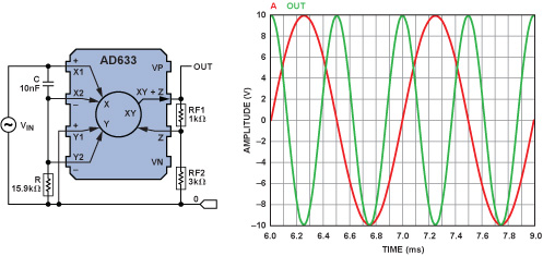
“Well, ah … maybe; though perhaps you should start with a bit of the history, going back to their earliest applications [15], and such basic questions as: What were electronic multipliers first used for during the WWII years—the late 1930s through to the mid-1940s? How did their value and use differ in the closing years of the 20th century? And in what ways was multiplication achieved prior to the advent of the translinear technique? Then provide examples of IC multipliers developed at ADI over the years, like the seminal and versatile AD534, with its innovative output-summing feature, the ‘Z’ pin, which surfaced later in an 8-pin IC, the AD633 (Figure 3).

“And of course, a review of this sort must mention the 10-MHz AD734—still the most accurate multiplier ever developed, by anyone, in any technology, other than the outdated and slow-as-molasses pulse-time-height [16] and hybrid multipliers, using DACs. There were early wideband multipliers, such as the AD834 and AD835, and then …”

“Whoa, Prof! … Don’t you think that’s rather a lot to cram into one article? I mean, isn’t its purpose to demonstrate the value of our newest parts for neurocomputers: like the ADNm22577 nanowatt analog array processor, the ADNm22585 order- statistics filter, or the ADNm22587 frame-capture correlator, all of which are used in Micha? Today’s readers will find these far more useful and can easily understand their functions. I’d really like to cut to the good stuff as quickly as possible!”

“Those are certainly valid concerns. But Nicky, keep in mind that the simple multipliers of the late 20^th and early 21^st century provided the foundation for what you are so expertly designing today. Don’t you think you should first say a bit about how they work? I’ll tell you what: I think I can rummage up a few lecture notes from the catacombs that you might wish to draw upon. We ought to have them readily at hand, anyway.”

With just a few gestures on the Actablet touch-panel/display that forms the glass top of every table at GalaxyBux, and the transparent connectivity of a campus-wide local net operating in the 35-GHz arena, supervised (and healed, when necessary) by neuromorphs like Michaday, Leif quickly located his old notes. He was relieved to discover that they still made good sense after so many years. “All right!! So, Mitch, please speak them,” he directed the Companion, who obliged, streaming via the Actablet to the pair’s permanently implanted earceivers, while Leif’s annotated text also scrolled on the TableScreen.

Solving Hard Equations in Real-Time

“Before neuromorphics,” began Michaday, “before binary computers of the sort that were in the ascendancy in the fifty years from 1960 to 2010, going back to World War II years, problems in mission-critical dynamical systems were solved using modeling techniques, with analog computing circuits, whose specific functions and connectivity embodied simultaneous (and often nonlinear) integro-differential equations. One simply let the network solve them—autonomously and asynchronously—and in some cases, interactively. Indeed, many such problems could only be solved by some kind of analogous device. This explains the 18^th– and 19^th-century fascination with mechanical differential analyzers [17], which very cleverly implemented summation/integration, addition/subtraction, and the like. As an aside, mainly because of noise considerations, the later electronic computers only sparingly used different initiators …”

“That’s differentiators, Micha,” chided Niku, chuckling.

“Sorry.” Continuing: “The structure of the equations determined the actual physical connections, which were often made at a patch panel, just like the manual telephone exchanges of the time. The fixed coefficients were set up in part as R-C time-constants, and in part by weighting factors, as gain or attenuation, sometimes using potentiometers. The equations also involved calculation of products (sometimes quotients) of the variables, all of which were represented by fairly high voltages … High voltages?! Oh … That’s not still true of me, is it?” quivered Michaday, who recalled having been terrified, during his installation days, by some sparks in a power unit that a negligent technician caused.

“Well … not so terribly large, in your case, Mitch,” joked Leif. “More like 25 millivolts. Actually, you use both voltage-mode and current-mode representations, whichever is appropriate at the functional level [19]. By the way, our human neurocircuits are just the same in this regard. Okay. Now, please proceed, and quit breaking the thread with self-indulgent observations!”

Niku hid an empathic grin behind her slender hand.

“Some of the nominally fixed coefficients may have needed to be altered, as the accuracy of the solution improved, using the potentiometers, which adjusted voltages acting on coefficient multipliers, and which were also of about a hundred volts full-scale,” gulped Michaday. “Do you wish me to continue?”

“Yes, Mitch, at least a couple more paragraphs.”

“Contrary to the popular myth, analog computers never died. They just went underground. All monolithic analog ICs—not just the multipliers—developed from 1965 onward, inherited the genes of those powerful early techniques. Thus, the term operational, as applied to an amplifier, declared that it was designed for the implementation of mathematical operations, such as integration or signal summation, ensuring as nearly as practicable that the function was solely a consequence of the external components, by placing full reliance on its (fairly) high open-loop gain, its (reasonably) low input offsets, and its (relatively) wide bandwidth.

“First-generation vacuum-tube op amps [18] were used by the thousands. Today, countless billions of virus-sized elements of their kind are doing much the same thing—with incomparably greater accuracy, speed, and efficiency. However, to multiply two variables was once a challenging quest; it required more than a few ‘linear’ op amps and external networks, due to the fundamental nature of this function. Many solutions devised at the time were hilariously crude by modern standards, scarcely up to the task. For example …”

“Okay, Micha,” interjected Niku. “Let’s pause here. Prof, as I see from the descriptions of the almost desperate methods used to approximate multiplication in the text that follows, their designers believed accuracies of 1% and bandwidths of a few kilohertz were regarded as the cat’s pajamas! We have come a long way! Some of the techniques that were concocted to do multiplication are scarcely credible. They’re in sharp contrast to the translinear principle that later was universally adopted for multiplication. It’s so very simple, inevitable, and elegant; even inherently obvious.”

“Heh! Perhaps that’s because I brainwashed you! But keep in mind that, for one thing, reliable silicon planar transistors, with their natural but gleefully fortuitous log-exponential properties, were decades into the future. What’s more, even the translinear multipliers of the last century had an Achilles’ heel: they were asymmetrical in the time-domain responses from their X and Y inputs, as well as in the linearity of these two signal paths. That remained a problem for some of the competition’s multipliers. Be sure to explain in your A-D article why time-symmetry and signal linearity are important. And, don’t leave the matter of quadrants of operation until too late in the piece.”

“I won’t. By the way, can you tell me where the labels, X and Y, used for a multiplier’s input ports, came from?”

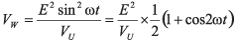
“No, I really don’t know when that first became the custom. Of course, they are commonly used for the two axes of a surface. Perhaps it was the choice of George Philbrick [20]. But I’m pretty sure that it was the Tinkerer who introduced today’s naming convention at ADI for the other variables associated with modern multiplier-dividers. I think it was at about the time the AD534 was being developed, which was the first analog multiplier designed expressly to be fully calibrated using laser-trimming at the wafer level. He used the notation

(1)

“The denominator voltage, V_U, was internally fixed at 10 V, using a buried Zener.³ The provision for adding in a further signal, V_Z, to the XY product was another of his innovations. It’s a rather nice example of the genesis of pragmatic novelty coming from thinking like the customer. You know, envisioning yourself slipping yourself into the shoes of several imaginary users of a new IC, persistently asking ‘In such-and-such a devious circumstance, what would I myself like this product to do?’ Here, while the main utility of the V_Z input was for adding a further variable to the product—for example, the output(s) of one or more other multipliers, as in correlation—the Tinkerer had much else in mind. I expect your article will explain its value in structuring a multiplier as a divider, and some of its many other uses.”

Niku said, enthusiastically: “Yes, of course! I remember now that this neat feature was found in almost all of the other multipliers designed by the Tinkerer. It also allowed several signals to be summed progressively simply by daisy-chaining the ‘next’ V_Z to the previous V_W … But, the wideband AD834 was a bit different, wasn’t it? As I recall, it had a differential current-mode output. But these can just as easily be summed, in an analog correlator, as I did recently in the ADNm22587, using directly paralleled output connections. However, the utility of that V_Z terminal goes far beyond such basic uses.”

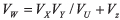
“Yes,” agreed Leif. “Remember this example? General-purpose multipliers were often used to square the amplitude of a signal. The X and Y ports received the same signal, V_IN, setting up the output V_W = V_IN²/V_U. Then, in the special case of a sinusoidal input, the output is a raised cosine at twice the frequency.

(2)

“In a 1976 article illustrating the numerous applications of the AD534 [21], the Tinkerer included a neat way to avoid that dc offset at the output, for a single frequency, without ac-coupling the output. He used just one CR network with ω₀ = 1/CR, and the two inputs were phase-shifted by +45° and –45°, with each attenuated by √2/2 at ω₀. Their 90° relative phase shift eliminates the output offset for inputs at ω₀ (see Figure 4).

(3)

“And here’s where the V_Z input served another useful function—not to add another signal to the output, in this case, but rather to raise the gain by a factor of 4, by feeding only a quarter of V_W to the Z pins, so realizing the full ±10-V output swing for a ±10-V sine input. This idea can also be implemented using an AD633, even though its 8-pin format limits the ‘Z’ function to just one pin (Figure 4). The ratio RF₂/(RF₂ + RF₁) determines the feedback factor. Of course, the frequency doesn’t have to be as low as 1 kHz, nor exactly 1/2πCR, and there are many things that can be done to reduce the variation of output amplitude over frequency. You might mention these in your article.”

“Hmm, it seems I will have to say quite a bit about all these ancient parts and their manifold applications in my article. By the way, I also read that article by the Tinkerer. It’s a terrific resource, but probably hard to find today. I was intrigued to discover how simple it is to synthesize novel functions using the normalized relationship, w = xy + z, where w = V_W/V_U, x = V_X/V_U, and so on. Constantly having to divide variables by that denominator is no fun, and nothing but a time-wasting distraction when you’re pursuing invention with just a Ziptip and a sketch-pad on your knee.”

“You’re right about the idea-enabling potential of w = xy + z, Nicky; but be careful never to fall into complacency about the importance of establishing and preserving scaling parameters in a nonlinear circuit. As a designer, whenever a scalar, such as V_U, appears in your target function, you’d better be absolutely sure you can vouch for it—that you are in full control of both its initial value and its environmentally threatened stability.”

“I certainly understand that’s something for us IC designers to worry about,” replied Niku. “But surely it’s less relevant for the user of the part. Can I rewind to an earlier point? All of today’s ‘vanilla’ multipliers operate in four quadrants. You know: V_W is the true algebraic product of V_X and V_Y, either of which may be positive or negative. But that wasn’t true of all those early IC multipliers you alluded to, was it?”

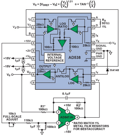
“No, it wasn’t. Our AD538, for example, was a ‘one-quadrant’ multiplier: it could only accept unipolar inputs at its X and Y ports. But the primary appeal of such parts was that they were usually more accurate at dc and low frequencies; and in addition, that one-of-a-kind AD538 had several other tricks up its sleeve, including multiple-decade operation, keying off the BJT’s wide-range log-exponential properties, as well as being able to generate both integral and fractional powers and roots of input signals and various less-common nonlinear functions.” (Figure 5 is an example of what Leif probably had in mind.)

“So … what about two-quadrant multiplication?” asked Niku.

“The AD538 could be connected to work in that fashion. But today, two-quadrant multipliers are more likely to be known as variable-gain amplifiers (VGAs). Their Y-channel desirably has low noise, very low distortion, and wide bandwidth, while the former X-channel is used to control the gain of that signal path.⁴ only a few multipliers optimized for gain control were developed, mostly during the mid-1970s. The 70-MHz AD539 was one such. That part featured dual, closely matched signal paths, for in-phase/quadrature (I/Q) signal processing.”

So … Aren’t VGAs Just Analog Multipliers?

“Prof, you once mentioned that it was the IC designers, rather than the user community, who first recognized that, in a VGA, the gain-control function is preferably linear in decibels—in other words, exponential—rather than linear in magnitude.”

“Right. Optimized VGAs actually are multipliers, in a certain sense, but they more usefully implement the function

(4)

“A₀ is simply the gain when x = 0. Recall that x = V_X/V_U, but V_U now represents something a bit different—although it’s still a very important reference voltage. If we focus on the gain as a function of x we have

(5)

(6)

reusing the variable, x, liberally rather than literally. The gain increases by a number of decibels proportional to V_X, with a slope (which may be gain-increasing or gain-decreasing, as either fixed or user-selectable modes) dependent on V_U.”

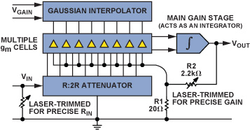
Niku said, “I recall that the Tinkerer gave the name X-AMP^® to his novel VGA topology (Figure 6), stressing that the ‘X’ doesn’t mean ‘experimental’ or ‘mysterious,’ but refers to the exponential aspect of the gain-control function. He and his team left a rich legacy of X-AMP devices, starting with the AD60x series, followed by the AD833x group, and, in modified form, the ADL5330. In other parts, such as the AD836x family, X-AMP was embedded into dc-to-GHz rms-responding measurement functions having true power-response even for microwaves, as well as in RF transceivers and demodulators.”

“True. And yet other ADI teams adopted the X-AMP idea, as in the 8-channel AD9271 X-AMP device, which included eight independent ADCs, for use in medical and industrial ultrasound. At the time of its introduction, it was regarded as state-of-the-art analog VLSI and won a ‘Product of the Year’ award in 2008. Really, these all were based on specialized spins of some sort of analog multiplier core; but we called ’em VGAs, as soon as that older, worn-out theme ran out of steam!” joked Leif.

“In fact,” he continued, “some of the voltage-controlled VGAs utilized a topology other than the X-AMP idea, harking back to the translinear-multiplier roots. While functioning as exponential amplifiers from a user’s perspective, internally they used the familiar current-mode gain-cells, augmented by elaborate and accurate circuitry for linear-in-dB gain-shaping.

“A classy example of an alternative form was the AD8330. Its core consisted of nothing more (well, perhaps a little bit more) than the four-transistor translinear multiplier, like this.” Leif pointed to a circuit on the Actablet, reproduced here as Figure 7. “The key idea is that the ratio of the currents in an input pair of transistors (Q1/Q2) forces the identical ratio of currents in the output pair (Q3/Q4). But those tail currents, I_D and I_N, are, in general, very different. The input current, I_IN (V_IN divided by the input resistance, R₁), is multiplied up or down by the ratio I_N/I_D, resulting in a linearly-amplified, current-mode output. This is converted back to voltage-mode by R_O, with a gain of (I_N/I_D)(R_O/R₁). The great appeal of this topology is that the shot noise of the input pair falls as the gain is increased, due to the reduction of the tail current, I_D.

“What makes the AD8330 so different is that I_A is arranged to be a temperature-stable exponential function of the primary (input-related) gain-control voltage, V_dBS, over a span of at least 50 dB, while on the other hand, I_B is simply proportional to a second (output-related) gain-control voltage, VLIN. This unique fusion of a ‘linear-in-dB’ VGA and ‘multiplier-style’ control of gain achieved, in effect, the combination of what the Tinkerer referred to as an ‘IVGA’—a VGA optimized to cope with a large dynamic range at its signal input—with an ‘OVGA,’ one optimized to provide a widely variable output amplitude. If the output’s gain-span was used in tandem with the input’s 50-dB gain-span, an unprecedented continuous gain-span of >115 dB could be realized, under the control of a single voltage.

“But the intrepid Tinkerer didn’t let it rest there. He solved one of the most pernicious problems of VGAs, namely, that the high-frequency response was invariably a strong function of the gain. At high gain settings, it tended to roll off—generally in a fairly benign way. But for low gains, most VGAs of that time eventually exhibited a strongly rising HF response. This problem was so severe in many competing products that at some high frequency above the specified bandwidth, the actual gain didn’t depend at all on the control voltage!”

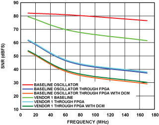
Niku said: “Yes, I remember once doing some measurements of my own, on a drawer-full of old samples in the lab, and saw this effect.  I also checked for myself the data-sheet claim that the AD8330 didn’t suffer from this problem at all.” Using the Actablet to locate her early work, she found Figure 8. “Ah-ha, here’s what I’m looking for. So … the left panel shows the HF response of the … should I mention the part’s manufacturer?”

“Better not,” Leif grinned broadly, “though they and a lot of other standard analog-IC outfits faltered in the early 2000s.”

“Okay. On the right is the AD8830’s frequency response. I was amazed by how closely all the samples met the data sheet’s promises. I’ve often wondered why it took so long for this part to become popular. It was a great little VGA, with good all-around specs and tremendous versatility, hiding a lot of deeply elegant design—not a bit like the simple repeated cells used in Michaday’s parallel-array processors and correlators …”

Niku was deliberately teasing Michaday—still remotely paying close attention to this flow of information, for possible future use. However, over at GalaxyBux, neither Niku nor Leif could see the expression on its animatrix face. While quite irrelevant to its function, this feature was often left in operation, for the amusement of visitors to the Michael Faraday auditorium, on ADI’s Solna campus. And if ever a neuromorph could ‘put on a pout,’ this would very aptly describe its visage just then. But due to a technical oversight, while he (or ‘she’?—apart from the masculine name, it could be either, or neither) could clearly see Leif and Niku, its facial views were not replicated in the down-link data to any of the remote Actablets. And today, a neuromorph’s capacity to interpret the expressions of humans is very good [23]. Initially, only the most rudimentary pattern-recognition tasks (such as “Is that a face, or a hot dog?”) were possible. However, Neuromorphics, Inc. machines are far more sensitive, and can discern the most subtle facial nuances. And, right there and then, Michaday wasn’t at all pleased by the conspiratorial grins that glimmered across the coffee cups.

“Excuse me … Will you be needing any further services, today? I am rather busy,” he said peevishly in their earceivers.

Leif said, “Alright, Mich, since you have managed to wriggle back into the story line, I’ll mention here that your multipliers are in fact not-so-ordinary, if for no other reason than they are quite unlike anything we have discussed. They use full-scale values of mere millivolts for their voltage-mode state-variables, and only a few nanoamps for current-mode variables. Such low-level representations are possible only because of the massively parallel nature of your hypercessors, the miles of your interconnects, and the sheer ameliorative power of abundant redundancy. As the term ‘neuromorphic’ implies, Mich, Companions like you are modeled on human systems, including this reliance on concurrency and parallelism. But what is probably much less well-known is that your state-variables are almost identical in magnitude to those found in organic neurons. You know, it’s an intriguing fact that …”

Neurons Are… Translinear!?

Here, Leif hesitated, weighing the imminence of mentioning an absolutely fascinating aspect of neural behavior against the risk of totally losing the ‘multiplier’ thread—which had already become slender. But, countenancing the fact that, sooner or later, the pivotal topic of the bipolar junction-transistor’s V_BE would have to be raised by Niku somewhere in her article, in order to explain translinear concepts from first principles, he leaned out far in the direction of indiscretion.

“Niku, you won’t need to mention this in your article, but there is this thing called Nernst’s Law [22], an important application of which is the quantification of the current-flow that diffuses across the cell membrane of a neuron, the key decision element found everywhere in living systems. The relationship is usually stated in terms of the variables of chemistry, rather than those of electronics. Consequently, I had to do a bit of speculation, at first, regarding the matter of its scaling dimensions; but the outcome of my research was gratifying.” (Figure 9.)

“I found that, in the chemistry of weak aqueous solutions of, say, sodium chloride, NaCl, the positively-charged Na⁺ ions can be regarded as roughly equivalent to the holes in the base of a transistor, while—rather more similarly—electrons are in correspondence to singly ionized Na^–. These are atoms, of course, but in the neuron, they are carriers of charge, much like holes and electrons, and they diffuse in concentration gradients.

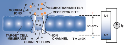
“Now, the question arises: for a given charge concentration on either side of the neuron’s cell membrane, what is the potential established across this barrier after ions have diffused across it to establish equilibrium? The answer, in chemistry—after one wakes up to the fact that an obscure scaling quantity, RT/Fzs, is just our old friend, kT/q, in disguise—is truly astonishing:

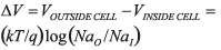(7)

“Here, Na_O and Na_I here are the sodium ion concentrations outside and inside the neuron respectively. In this respect, the neuron is behaving very much like the delta-V_BE of a BJT! It even exhibits a slope, roughly equivalent to the transistor’s transconductance! Not just some vague transconductance like the old CMOS transistors, but one just like a modern BJT: one that is linear with a concentration gradient—a current-density, a current flow! So is it putting too fine a sheen on all this, to view neurons as translinear elements?

“The underlying physical principles are the same: both involve similar processes of diffusion and mobility; both conform to Fick’s equation and invoke the Einstein relationship, familiar to semiconductor specialists. Since this aspect of the behavior of a neuron so closely parallels that of a semiconductor device, it should not be surprising that this same relationship is used over and over again in the neuromorphic decision elements of Michaday as well as in most of your recent ICs, Niku. Consider this: for an ion ratio of 10 in the cell of Figure 9, the membrane potential in a neuron is 61.5 mV!”

“All this is fascinating! But, wait a minute. Wouldn’t a charge concentration ratio of 10 generate 59.525 mV, proportional to absolute temperature: PTAT, to use the Tinkerer’s term? [24]”

“Nicky, I have never been inclined to call you a ‘hot-head’… but your brain operates at 310 K. The value of 25.85 mV for kT/q is for an assumed temperature of 300 K, close to 27°C. In our bodies, kT/q is (310/300) × 25.85 mV, so for an ion ratio of 10, the human neuronal difference potential is 61.51 mV.”

“Of course! Still … might a better comparison to the neuron be, say, a multiple-gate MOS transistor operating in subthreshold? I mean … a neuron has this capacity for linear multiplication, based on its translinear qualities, but it also can perform such things as integration, even with recursion, signal summation with discretionary weighting—all the functions that are at the heart of solving equations in analog computers! It’s no wonder that today’s neurocomputers are so powerfully intelligent! And I can see clearly now—after having worked with you these past months—why you’re always so passionate about stressing the ‘Fundaments.’ It really is crucial to have a firm grasp on all of them, and be aware of interdisciplinary truths like these.

“By the way, Prof, I’ve been doing a bit of my own research … well, with Micha’s help …” (was that a sigh of appreciation in the downlink?) “and I found that the Tinkerer anticipated the future relevance of translinear elements to neural hardware as far back as 1988, 40 years ago! During his presentation at the first Workshop on Neural Hardware [25] in San Diego, he predicted today’s nanowatt computing elements, the role of translinear concepts, and he even noted Nernst’s Law and its astonishing similarity to the equation for the key voltage-current relationship in a BJT—the same rock-solid foundation of translinear theory. Micha’s just located for me a 1990 essay by him [26] in which he observed that, just as carrier injection at the emitter-base of a BJT is affected by quantum fluctuations in the band energies, thus generating shot noise,⁵ so likewise must neurons be affected. He said it’s lucky for us that neurons are not entirely deterministic, since we’d be very dull people!”

“I also learned that in any cluster of neurons, there are multiple feedback paths, like those sometimes associated with op amp circuitry, and many of them are nonlinear, too. It seems this is the fertile soil from which sprouts chaotic behavior in neurons, which is quasi-deterministic, leading to the original thought. The Tinkerer argued that human creativity actually depends on moderate amounts of stochastic noise—and that idea would go a long way toward explaining the ephemeral, unpredictable quality of the sudden flash of insight. Isn’t that a hoot!?”

“Well, Niku,” said the elder, “between us, we’ve drifted a long way from the topic of analog multipliers! Tell you what. I have a three-PM with the Director, and it’s getting close to that time, so why don’t you finish up your ideas for your next A-D article back in the lab? I’m really looking forward to seeing it!”

Leif and Niku rose from the still-glowing Actablet and strolled to the door. The unfailingly-irritating GalaxyBux AutoGreeter opened it, and the disembodied voice said, in that cheery, ding-dong fashion “Glad to be of ser-vice to you!” They exchanged a giggly glance. “See how far the science of neuromemics has gotten us!” joked Leif. Lacking ears (they assumed, as being irrelevant to its prosaic function) the Greeter had nothing more to say … just then, anyway.

(to be continued)

END NOTES

^†Information and data sheets on all products mentioned here may be found on the Analog Devices website, http://www.analog.com.

¹From “meme,” the unit of imitation [8]; used in this adjectival way since 2018.

²See D-Day; The Wit and Wisdom of Dr. Leif [Analog Dialogue 40-3, p. 3.]

³An idea he imported into ADI, during the mid-1970s, but revealed to him, without preconditions, by Bob Dobkin, later of LTC, during a long, aprés-ISSCC bar-chat.

⁴By the Tinkerer’s convention, wherever this distinction arose, “Y” was used for the more linear “signal-oriented” path, while “X” referred to the slower, and either less-critically linear, or in some cases deliberately nonlinear, gain-control function. This naming convention evaporated as general-purpose multipliers slowly morphed first into general-purpose VGAs and then into even more specialized types.

⁵Leif says it’s improperly called “collector shot noise,” because it’s due principally to statistical fluctuations at the emitter junction. These variations in the mean current travel across the base to the collector junction (which is not a barrier, but more like a waterfall). Some extra noise might be generated here, but only when the field strength is high enough to cause ionization (avalanche multiplication).

参阅电路

[1] Gilbert, B. “A DC-500 MHz Amplifier/Multiplier Principle.” ISSCC Technical Digest. Feb 1968. pp. 114–115. This was the first public disclosure of circuits exploiting what later would be called “The Translinear Principle.” [3]

[2] Gilbert, B. “A Precise Four-Quadrant Multiplier with Subnanosec ond Response.” IEEE Jour. Solid State Circuits, Vol. SC-3, No. 4. pp. 365–373.

[3] Gilbert, B. “Translinear Circuits: A Proposed Classification.” Electron Lett., Vol. 11, No. 1. pp. 14–16. Jan 1975.

[4] Gilbert, B. “Translinear Circuits: An Historical Overview.” Analog Integrated Circuits and Signal Processing 9-2. Mar 1996. pp. 95–118.

[5] Toumazou, C., G. Moschytz, B. Gilbert, and G. Kathiresan. Trade-Offs in Analog Circuit Design, The Designer’s Companion, Part Two. Springer US. 2002. ISBN 978-1-4020-7037-2.

[6] Gilbert, B. “The Multi-tanh Principle: A Tutorial Overview.” IEEE Jour. Solid-State Circuits, 33-1. 1998. pp. 2–17.

[7] KERMIT, meaning “Kommon-EmitteR MultI-Tanh”, is an extremely versatile cell form, in which N > 2 emitters (or sources) are joined and supplied with one current-source. An early example (though not yet named that) appears as the vector scanner, in the paper: “Monolithic analog read-only memory for character generation,” by Gilbert, B. IEEE J. Solid-State Circuits, Vol. SC-6, No. 1. pp. 45–55. 1971.

[8] Blackmore, Susan. The Meme Machine. Oxford University Press. 1999. ISBN 0-19-286212-X. An excellent introduction to the idea of memetic growth.

[9] Powell, J. R. “The Quantum Limit to Moore’s Law.” Proc. IEEE, Vol. 96, No. 8. Aug 2008. pp 1247–48.

[10] Gilbert, B. A monolithic 16-channel analog array normalizer.” IEEE Jour. Solid-State Circuits, 19-6. Dec 1984. pp. 956–63.

[11] Gilbert, B. “A New Technique for Analog Multiplication.” IEEE Jour. Solid State Circuits, 10-6. Dec 1975. pp. 437–47.

[12] Gilbert, B. “A Super-Integrated 4-Decade Counter with Buffer Memory and D/A Output Converters.” ISSCC Tech Digest. 1970. pp 120–121.

[13] Wiedmann, S. K. “High-Density Static Bipolar Memory.” ISSCC Tech. Digest. 1973. pp. 56–57.

[14] Gilbert, B. “Novel Magnetic-Field Sensor using Carrier Rotation.” Electronics Letters, Vol. 12, No. 31. Nov 1976. pp 608–611.

[15] Paynter, H. M., ed. A Palimpsest on the Electronic Art (Being a collection of reprints of papers & other writings which have been in demand over the past several years). 1955. Boston: George A. Philbrick Researches, Inc. Fascinating, authoritative, and relevant to this day. Although long out of print, it is worth seeking out on eBay.

[16] Korn, G.A., and T.M. Korn. Electronic Analog Computers. NY:  McGraw Hill Book Company. 1952.

[17] For an extensive history, see http://everything2.com/e2node/Differential%2520analyzer. For an intriguing account of a differential analyzer built with Meccano, see www.dalefield.com/nzfmm/magazine/Differential_Analyser.html

[18] Gilbert, B. “Current Mode, Voltage Mode, or Free Mode? A Few Sage Suggestions.” Analog Integrated Circuits and Signal Processing, Vol. 38, Nos. 2-3, Feb 2004. pp. 83–101.

[19] A fragment of an early article about ‘Analog Computors,’ written by G.A. Philbrick, can be found at http://www.philbrickarchive.org/dc032_philbrick_history.htm

[20] X,Y,Z and W were used in specifying the Philbrick SK5-M four-quadrant multiplier, but in the form W = XY/Z, rather than the later usage W = XY/U + Z. See  www.philbrickarchive.org/sk5-m.htm. Incidentally, this magnificent machine needed 200 W to light it up!

[21] Gilbert, B. “New Analogue Multiplier Opens Way to Powerful Function Synthesis.” Microelectronics. Vol. 8, No. 1. pp 26–36. 1976. May be hard to find, but Niku dips into her copy in Part 2.

[22] Aityan, S.K. and C. Gudipalley. “Image Understanding with Intelligent Neural Networks.” World Congress on Neural Networks. Portland, OR. Jun 1993. Vol. 1. pp 518–523. A milestone event. Other papers in this extensive five-volume resource will be of interest to anyone interested in the status of neuroelectronics in the early 1990s.

[23] Partridge, Lloyd D. and L. Donald. The Nervous System. MIT Press. 1992. ISBN 0-262-16134-6. This is a very well-written book, providing an excellent introduction for the electronics engineer to the design and function of neurons. Appendix I derives Nernst’s Law from the starting point of ionic diffusion in a weak solution.

[24] The abbreviation ‘PTAT’ was first used in Section B (p. 854) of the paper by Gilbert, B, “A Versatile Monolithic Voltage-to-Frequency Converter,” Jour. Solid-State Circuits. Vol. 11. No. 6. Dec 1976, pp. 852-864.

[25] Gilbert, B. “Nanopower Nonlinear Circuits based on The Translinear Principle.” In workshop notes Hardware Implementation of Neuron Nets and Synapses. First Workshop on Neural Hardware. San Diego. Jan 1988. pp. 135–170.

[26] Coming Next Week! The Elements of Innovention. An early version of this rambling essay, concerning the root sources of creativity, was mounted without the author’s permission on the Internet during the mid-1990s. An update is available from barrie.gilbert@analog.com.